Dimensionality Reduction
Dimensionality Reduction
Fitting and overfitting get worse with ''curse of dimensionality'' Bellman 1961
Think about a hypersphere. Its volume is given by
\begin{equation} V_D(r) = \frac{2r^D\pi^{D/2}}{D\ \Gamma(D/2)}, \end{equation}where $\Gamma(z)$ is the complete gamma function, $D$ is the dimension, and $r$ the radius of the sphere.
If you populated a hypercube of size $2r$ how much data would be enclosed by the hypersphere
- as $D$ increases the fractional volume enclosed by the hypersphere goes to 0!
For example: the SDSS comprises a sample of 357 million sources.
- each source has 448 measured attributes
- selecting just 30 (e.g., magnitude, size..) and normalizing the data range $-1$ to $1$
probability of having one of the 357 million sources reside within a unit hypersphere 1 in 1.4$\times 10^5$.
%matplotlib inline
import numpy as np
import scipy.special as sp
from matplotlib import pyplot as plt

def unitVolume(dimension, radius=1.):
    return 2*(radius**dimension *np.pi**(dimension/2.))/(dimension*sp.gamma(dimension/2.))

dim = np.linspace(1,100)

#------------------------------------------------------------
# Plot the results
fig = plt.figure()
ax = fig.add_subplot(111)
ax.plot(dim,unitVolume(dim)/2.**dim)

ax.set_yscale('log')
ax.set_xlabel('$Dimension$')
ax.set_ylabel('$Volume$')

plt.show()

D=2;unitVolume(D)/(2.**D)
What can we do to reduce the dimensions
Principal component analysis or the Karhunen-Loeve transform
The first refuge of a scoundrel...

Points are correlated along a particular direction which doesn't align with the initial choice of axes.
- we should rotate our axes to align with this correlation.
- rotation preserves the relative ordering of data
Choose rotation to maximize the ability to discriminate between the data points
- first axis, or principal component, is direction of maximal variance
- second principal component is orthogonal to the first component and maximizes the residual variance
- ...
Derivation of principal component analyses
Set of data $X$: $N$ observations by $K$ measurements
Center data by subtracting the mean
The covariance is
$ C_X=\frac{1}{N-1}X^TX, $
$N-1$ as the sample covariance matrix
We want a projection, $R$, aligned with the directions of maximal variance ($Y= X R$) with covariance
$ C_{Y} = R^T X^T X R = R^T C_X R $
Derive principal component by maximizing its variance (using Lagrange multipliers and constraint)
$ \phi(r_1,\lambda_1) = r_1^TC_X r_1 - \lambda_1(r_1^Tr_1-1). $
derivative of $\phi(r_1,\lambda)$ with respect to $r_1$ set to 0
$ C_Xr_1 - \lambda_1 r_1 = 0. $
$\lambda_1$ is the root of the equation $\det(C_X - \lambda_1 {\bf I})=0$ and the largest eigenvalue
$ \lambda_1 = r_1^T C_X r_1 $
Other principal components derived by applying additional constraint that components are uncorrelated (e.g., $r^T_2 C_X r_1 = 0$).
Computation of principal components
Common approach is eigenvalue decomposition of the covariance or correlation matrix, or singular value decomposition (SVD) of the data matrix
SVD given by
$ U \Sigma V^T = \frac{1}{\sqrt{N - 1}} X, $
columns of $U$ are left-singular vectors
columns of $V$ are the right-singular vectors
The columns of $U$ and $V$ form orthonormal bases ($U^TU = V^TV = I$)
Covariance matrix is
$ \begin{eqnarray} C_X &=& \left[\frac{1}{\sqrt{N - 1}}X\right]^T \left[\frac{1}{\sqrt{N - 1}}X\right]\nonumber\ &=& V \Sigma U^T U \Sigma V^T\nonumber\ &=& V \Sigma^2 V^T. \end{eqnarray} $
right singular vectors $V$ are the principal components so principal from the SVD of $X$ dont need $C_X$.
Preparing data for PCA
- Center data by subtracting the mean of each dimension
- For heterogeneous data (e.g., galaxy shape and flux divide by variance (whitening).
- For spectra or images normalize each row so integrated flux of each object is one.
import numpy as np
from matplotlib import pyplot as plt

from sklearn.decomposition import PCA
from sklearn.decomposition import RandomizedPCA

from astroML.datasets import sdss_corrected_spectra
from astroML.decorators import pickle_results

#------------------------------------------------------------
# Download data
data = sdss_corrected_spectra.fetch_sdss_corrected_spectra()
spectra = sdss_corrected_spectra.reconstruct_spectra(data)
wavelengths = sdss_corrected_spectra.compute_wavelengths(data)


#----------------------------------------------------------------------
# Compute PCA
def compute_PCA(n_components=5):
#    np.random.seed(500)
    nrows = 500
    ind = np.random.randint(spectra.shape[0], size=nrows)

    spec_mean = spectra[ind].mean(0)
#    spec_mean = spectra[:50].mean(0)

    # PCA: use randomized PCA for speed
    pca = PCA(n_components - 1)
    pca.fit(spectra[ind])
    pca_comp = np.vstack([spec_mean,
                          pca.components_])
    evals = pca.explained_variance_ratio_

    return pca_comp, evals

n_components = 5
decompositions, evals = compute_PCA(n_components)

#----------------------------------------------------------------------
# Plot the results
fig = plt.figure(figsize=(10, 8))
fig.subplots_adjust(left=0.05, right=0.95, wspace=0.05,
                    bottom=0.1, top=0.95, hspace=0.05)

titles = 'PCA components'

for j in range(n_components):
    ax = fig.add_subplot(n_components, 2, 2*j+2)

    ax.yaxis.set_major_formatter(plt.NullFormatter())
    ax.xaxis.set_major_locator(plt.MultipleLocator(1000))
    if j < n_components - 1:
        ax.xaxis.set_major_formatter(plt.NullFormatter())
    else:
        ax.set_xlabel(r'wavelength ${\rm (\AA)}$')
    ax.plot(wavelengths, decompositions[j], '-k', lw=1)

    # plot zero line
    xlim = [3000, 7999]
    ax.plot(xlim, [0, 0], '-', c='gray', lw=1)
    ax.set_xlim(xlim)

    # adjust y limits
    ylim = plt.ylim()
    dy = 0.05 * (ylim[1] - ylim[0])
    ax.set_ylim(ylim[0] - dy, ylim[1] + 4 * dy)


    ax2 = fig.add_subplot(n_components, 2, 2*j+1)
    ax2.yaxis.set_major_formatter(plt.NullFormatter())
    ax2.xaxis.set_major_locator(plt.MultipleLocator(1000))
    if j < n_components - 1:
        ax2.xaxis.set_major_formatter(plt.NullFormatter())
    else:
        ax2.set_xlabel(r'wavelength ${\rm (\AA)}$')
    ax2.plot(wavelengths, spectra[j], '-k', lw=1)

    # plot zero line
    ax2.plot(xlim, [0, 0], '-', c='gray', lw=1)
    ax2.set_xlim(xlim)

    if j == 0:
        ax.set_title(titles, fontsize='medium')

    if j == 0:
        label = 'mean'
    else:
        label = 'component %i' % j

    # adjust y limits
    ylim = plt.ylim()
    dy = 0.05 * (ylim[1] - ylim[0])
    ax2.set_ylim(ylim[0] - dy, ylim[1] + 4 * dy)


    ax.text(0.02, 0.95, label, transform=ax.transAxes,
            ha='left', va='top', bbox=dict(ec='w', fc='w'),
            fontsize='small')


plt.show()

import numpy as np
from matplotlib import pyplot as plt

#----------------------------------------------------------------------
# Plot the results
fig = plt.figure(figsize=(8, 4))

ax = fig.add_subplot(121)
ax.plot(np.arange(n_components-1), evals)
ax.set_xlabel("eigenvalue number")
ax.set_ylabel("eigenvalue ")

ax = fig.add_subplot(122)
ax.plot(np.arange(n_components-1), evals.cumsum())
ax.set_xlabel("eigenvalue number")
ax.set_ylabel("cumulative eigenvalue ")

plt.show()

Interpreting the PCA
Reconstruction of spectrum, ${x}(k)$, from the eigenvectors, ${e}_i(k)$
$ \begin{equation} {x}i(k) = {\mu}(k) + \sum_j^R \theta{ij} {e}_j(k), \end{equation} $
Truncating this expansion (i.e., $r $\begin{equation}
{x}_i(k) = {\mu}(k) + \sum_i^{r<R} \theta_i {e}_i(k),
\end{equation}
$ This is the sense in which PCA gives for dimensionality reduction.
import numpy as np
from matplotlib import pyplot as plt

from sklearn.decomposition import PCA

from astroML.datasets import sdss_corrected_spectra
from astroML.decorators import pickle_results

#------------------------------------------------------------
# Download data
data = sdss_corrected_spectra.fetch_sdss_corrected_spectra()
spectra = sdss_corrected_spectra.reconstruct_spectra(data)
wavelengths = sdss_corrected_spectra.compute_wavelengths(data)

#------------------------------------------------------------
# Compute PCA components

# Eigenvalues can be computed using PCA as in the commented code below:

#from sklearn.decomposition import PCA
#pca = PCA()
#pca.fit(spectra)
#evals = pca.explained_variance_ratio_
#evals_cs = evals.cumsum()

#  because the spectra have been reconstructed from masked values, this
#  is not exactly correct in this case: we'll use the values computed
#  in the file compute_sdss_pca.py
evals = data['evals'] ** 2
evals_cs = evals.cumsum()
evals_cs /= evals_cs[-1]
evecs = data['evecs']
spec_mean = spectra.mean(0)

#------------------------------------------------------------
# Find the coefficients of a particular spectrum
spec = spectra[1]
coeff = np.dot(evecs, spec - spec_mean)

#------------------------------------------------------------
# Plot the sequence of reconstructions
fig = plt.figure(figsize=(8, 8))
fig.subplots_adjust(hspace=0)

for i, n in enumerate([0, 4, 8, 20]):
    ax = fig.add_subplot(411 + i)
    ax.plot(wavelengths, spec, '-', c='gray')
    ax.plot(wavelengths, spec_mean + np.dot(coeff[:n], evecs[:n]), '-k')

    if i < 3:
        ax.xaxis.set_major_formatter(plt.NullFormatter())

    ax.set_ylim(-2, 21)
    ax.set_ylabel('flux')

    if n == 0:
        text = "mean"
    elif n == 1:
        text = "mean + 1 component\n"
        text += r"$(\sigma^2_{tot} = %.2f)$" % evals_cs[n - 1]
    else:
        text = "mean + %i components\n" % n
        text += r"$(\sigma^2_{tot} = %.2f)$" % evals_cs[n - 1]

    ax.text(0.01, 0.95, text, ha='left', va='top', transform=ax.transAxes)

fig.axes[-1].set_xlabel(r'${\rm wavelength\ (\AA)}$')
plt.show()

- Comparisons between the eigenvectors derived from PCA and known spectral types of galaxies have shown that these statistically orthogonal components correlate strongly with specific physical properties
- given the cumulative nature of the sum of variances used in PCA, astrophysically interesting components within the spectra (e.g., sharp spectral lines or transient features for certain galaxy populations) may not be reflected in the largest PCA components.
- sum of linear components can efficiently reconstruct the features within the data does not always hold. An example of this is the variation in broad emission lines (such as those from quasars). The variation in line width is an inherently nonlinear process and can require a large number of components to fully characterize: for broad line quasars over 30 components are required to reproduce the underlying spectra compared to the 10 required for quiescent and star-forming galaxies.
PCA with missing data
Observed spectrum, $x^o$ is the true spectrum, ${x}$ plus a wavelength-dependent weight, ${w}$.
Weight is zero where data are missing and $1/{\sigma}^2$ for rest
Minimizing the quadratic deviation between ${x}^o$ truncated reconstruction, $\sum_i \theta_i {e}_i$ and solving for $\theta_i$ gives
$\begin{equation} \sum_k \theta_i {w}(k) {e}_i(k) {e}_j(k) = \sum_k {w}(k) {x}^o(k) {e}_j(k), \end{equation} $
If $M_{ij} = \sum_k {w}(k) {e}_i(k) {e}_j(k)$ and $F_i = \sum_k {w}(k) {x}^o(k) {e}_i(k)$ then
$\begin{equation} \thetai = \sum_j M{ij}^{-1} F_{j}, \end{equation} $
- $F_j$ are coefficients derived from gappy data
- $M_{ij}^{-1}$ shows how correlated eigenvectors are over the missing regions.
An estimate of the uncertainty on the reconstruction coefficients is given by
$\begin{equation} %Cov(\thetai,\theta_j) = \frac{1}{N}M{ij}^{-1} {\rm Cov}(\thetai,\theta_j) = M{ij}^{-1}. \end{equation} $
Accuracy of this reconstruction will depend on the distribution of the gaps within the data vector.
import numpy as np
from matplotlib import pyplot as plt
from matplotlib import ticker

from astroML.datasets import fetch_sdss_corrected_spectra
from astroML.datasets import sdss_corrected_spectra

#------------------------------------------------------------
# Get spectra and eigenvectors used to reconstruct them
data = fetch_sdss_corrected_spectra()
spec = sdss_corrected_spectra.reconstruct_spectra(data)
lam = sdss_corrected_spectra.compute_wavelengths(data)
evecs = data['evecs']
mu = data['mu']
norms = data['norms']
mask = data['mask']

#------------------------------------------------------------
# plot the results
i_plot = ((lam > 5750) & (lam < 6350))
lam = lam[i_plot]

specnums = [20, 8, 9]
subplots = [311, 312, 313]

fig = plt.figure(figsize=(8, 10))
fig.subplots_adjust(hspace=0)

for subplot, i in zip(subplots, specnums):
    ax = fig.add_subplot(subplot)

    # compute eigen-coefficients
    spec_i_centered = spec[i] / norms[i] - mu
    coeffs = np.dot(spec_i_centered, evecs.T)

    # blank out masked regions
    spec_i = spec[i]
    mask_i = mask[i]
    spec_i[mask_i] = np.nan

    # plot the raw masked spectrum
    ax.plot(lam, spec_i[i_plot], '-', color='k', lw=2,
            label='True spectrum')

    # plot two levels of reconstruction
    for nev in [10]:
        if nev == 0:
            label = 'mean'
        else:
            label = 'nev=%i' % nev
        spec_i_recons = norms[i] * (mu + np.dot(coeffs[:nev], evecs[:nev]))
        ax.plot(lam, spec_i_recons[i_plot], label=label)

    # plot shaded background in masked region
    ylim = ax.get_ylim()
    mask_shade = ylim[0] + mask[i][i_plot].astype(float) * ylim[1]
    plt.fill(np.concatenate([lam[:1], lam, lam[-1:]]),
             np.concatenate([[ylim[0]], mask_shade, [ylim[0]]]),
             lw=0, fc='k', alpha=0.2)

    ax.set_xlim(lam[0], lam[-1])
    ax.set_ylim(ylim)
    ax.yaxis.set_major_formatter(ticker.NullFormatter())

    if subplot == 311:
        ax.legend(loc=1, prop=dict(size=14))

    ax.set_xlabel('$\lambda\ (\AA)$')
    ax.set_ylabel('normalized flux')

plt.show()

Non negative factorization
Eigenvectors are defined relative to mean data vector. Principal components that can be positive or negative but for many physical systems we know data are a linear sum of positive components (e.g. galaxy spectrum is a linear sum of stellar components
Nonnegative matrix factorization (NMF) applies positivity constraint
Assumes any data matrix can be factored into two matrices, $W$ and $Y$, with
$\begin{equation} X=W Y, \end{equation} $
and both $W$ and $Y$ are nonnegative
$WY$ is an approximation of $X$. Minimizing the reconstruction error $|| (X - W Y)^2 ||$ nonnegative bases can be derived using a simple update rule,
$ \begin{eqnarray} W{ki} &=& W{ki}\frac{[XY^T]{ki}}{[WYY^T]{ki}},\ Y{in} &=& Y{in}\frac{[W^TX]{in}}{[W^TWY]{in}}, \end{eqnarray} $
Iterative process does not guarantee nonlocal minima (like $K$-means and EM).
Use random initialization and cross-validation
# Author: Jake VanderPlas
# License: BSD
%matplotlib inline

import numpy as np
from matplotlib import pyplot as plt

from sklearn.decomposition import NMF
from sklearn.decomposition import RandomizedPCA

from astroML.datasets import sdss_corrected_spectra
from astroML.decorators import pickle_results

#----------------------------------------------------------------------
# This function adjusts matplotlib settings for a uniform feel in the textbook.
# Note that with usetex=True, fonts are rendered with LaTeX.  This may
# result in an error if LaTeX is not installed on your system.  In that case,
# you can set usetex to False.
from astroML.plotting import setup_text_plots
setup_text_plots(fontsize=8, usetex=True)

#------------------------------------------------------------
# Download data
data = sdss_corrected_spectra.fetch_sdss_corrected_spectra()
spectra = sdss_corrected_spectra.reconstruct_spectra(data)
wavelengths = sdss_corrected_spectra.compute_wavelengths(data)


#----------------------------------------------------------------------
# Compute PCA, and NMF components
#  we'll save the results so that they can be re-used
@pickle_results('spec_decompositions.pkl')
def compute_PCA_NMF(n_components=5):
    spec_mean = spectra.mean(0)

    # PCA: use randomized PCA for speed
    pca = RandomizedPCA(n_components - 1)
    pca.fit(spectra)
    pca_comp = np.vstack([spec_mean,
                          pca.components_])


    # NMF requires all elements of the input to be greater than zero
    spectra[spectra < 0] = 0
    nmf = NMF(n_components)
    nmf.fit(spectra)
    nmf_comp = nmf.components_

    return pca_comp, nmf_comp

n_components = 5
decompositions = compute_PCA_NMF(n_components)

#----------------------------------------------------------------------
# Plot the results
fig = plt.figure(figsize=(10, 10))
fig.subplots_adjust(left=0.05, right=0.95, wspace=0.05,
                    bottom=0.1, top=0.95, hspace=0.05)

titles = ['PCA components', 'NMF components']

for i, comp in enumerate(decompositions):
    for j in range(n_components):
        ax = fig.add_subplot(n_components, 3, 3 * j + 1 + i)

        ax.yaxis.set_major_formatter(plt.NullFormatter())
        ax.xaxis.set_major_locator(plt.MultipleLocator(1000))
        if j < n_components - 1:
            ax.xaxis.set_major_formatter(plt.NullFormatter())
        else:
            ax.set_xlabel(r'wavelength ${\rm (\AA)}$')

        ax.plot(wavelengths, comp[j], '-k', lw=1)

        # plot zero line
        xlim = [3000, 7999]
        ax.plot(xlim, [0, 0], '-', c='gray', lw=1)
        ax.set_xlim(xlim)

        if j == 0:
            ax.set_title(titles[i])

        if titles[i].startswith('PCA') or titles[i].startswith('ICA'):
            if j == 0:
                label = 'mean'
            else:
                label = 'component %i' % j
        else:
            label = 'component %i' % (j + 1)

        ax.text(0.03, 0.94, label, transform=ax.transAxes,
                ha='left', va='top')

        for l in ax.get_xticklines() + ax.get_yticklines():
            l.set_markersize(2)

        # adjust y limits
        ylim = plt.ylim()
        dy = 0.05 * (ylim[1] - ylim[0])
        ax.set_ylim(ylim[0] - dy, ylim[1] + 4 * dy)


plt.show()

Manifold Learning
Real-world data sets often have very nonlinear features (e.g. QSOs with broad lines) which are hard to describe compactly using linear eigenvectors. Manifold learning techniques search for a representation of these data within a lower dimensional space
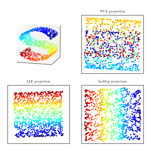
Local Linear Embedding:
Step 1: define local geometry
- local neighborhoods determined from $k$ nearest neighbors.
- for each point calculate weights that reconstruct a point from its $k$ nearest
neighbors
$ \begin{equation} \mathcal{E}_1(W) = \left|X - WX\right|^2 \end{equation} $
- essentially this is finding the hyperplane that describes the local surface at each point within the data set.
Step 2: embed within a lower dimensional space
- set all $W_{ij}=0$ except when point $j$ is one of the $k$ nearest neighbors of point $i$.
- $W$ becomes very sparse for $k \ll N$.
- minimize
$\begin{equation} \mathcal{E}_2(Y) = \left|Y - W Y\right|^2, \end{equation} $
with $W$ fixed to find an $N$ by $d$ matrix ($d$ is the new dimensionality)
Step 1 requires a nearest-neighbor search.
Step 2 requires an eigenvalue decomposition of the matrix $C_W \equiv (I-W)^T(I-W)$,
LLE has been applied to data as diverse as galaxy spectra, stellar spectra, and photometric light curves.
# Author: Jake VanderPlas
# License: BSD
import numpy as np
from matplotlib import pyplot as plt
from sklearn import manifold, neighbors

from astroML.datasets import sdss_corrected_spectra
from astroML.datasets import fetch_sdss_corrected_spectra
from astroML.plotting.tools import discretize_cmap
from astroML.decorators import pickle_results

#----------------------------------------------------------------------
# This function adjusts matplotlib settings for a uniform feel in the textbook.
# Note that with usetex=True, fonts are rendered with LaTeX.  This may
# result in an error if LaTeX is not installed on your system.  In that case,
# you can set usetex to False.
from astroML.plotting import setup_text_plots
setup_text_plots(fontsize=8, usetex=True)

#------------------------------------------------------------
# Set up color-map properties
clim = (1.5, 6.5)
cmap = discretize_cmap(plt.cm.jet, 5)
cdict = ['unknown', 'star', 'absorption galaxy',
         'galaxy', 'emission galaxy',
         'narrow-line QSO', 'broad-line QSO']
cticks = [2, 3, 4, 5, 6]
formatter = plt.FuncFormatter(lambda t, *args: cdict[int(np.round(t))])


#------------------------------------------------------------
# Fetch the data; PCA coefficients have been pre-computed
data = fetch_sdss_corrected_spectra()
coeffs_PCA = data['coeffs']
c_PCA = data['lineindex_cln']
spec = sdss_corrected_spectra.reconstruct_spectra(data)
color = data['lineindex_cln']


#------------------------------------------------------------
# Compute the LLE projection; save the results
@pickle_results("spec_LLE.pkl")
def compute_spec_LLE(n_neighbors=10, out_dim=3):
    # Compute the LLE projection
    LLE = manifold.LocallyLinearEmbedding(n_neighbors, out_dim,
                                          method='modified',
                                          eigen_solver='dense')
    Y_LLE = LLE.fit_transform(spec)
    print " - finished LLE projection"

    # remove outliers for the plot
    BT = neighbors.BallTree(Y_LLE)
    dist, ind = BT.query(Y_LLE, n_neighbors)
    dist_to_n = dist[:, -1]
    dist_to_n -= dist_to_n.mean()
    std = np.std(dist_to_n)
    flag = (dist_to_n > 0.25 * std)
    print " - removing %i outliers for plot" % flag.sum()

    return Y_LLE[~flag], color[~flag]

coeffs_LLE, c_LLE = compute_spec_LLE(10, 3)


#----------------------------------------------------------------------
# Plot the results:
for (c, coeffs, xlim) in zip([c_PCA, c_LLE],
                             [coeffs_PCA, coeffs_LLE],
                             [(-1.2, 1.0), (-0.01, 0.014)]):
    fig = plt.figure(figsize=(5, 3.75))
    fig.subplots_adjust(hspace=0.05, wspace=0.05)

    # axes for colorbar
    cax = plt.axes([0.525, 0.525, 0.02, 0.35])

    # Create scatter-plots
    scatter_kwargs = dict(s=4, lw=0, edgecolors='none', c=c, cmap=cmap)

    ax1 = plt.subplot(221)
    im1 = ax1.scatter(coeffs[:, 0], coeffs[:, 1], **scatter_kwargs)
    im1.set_clim(clim)
    ax1.set_ylabel('$c_2$')

    ax2 = plt.subplot(223)
    im2 = ax2.scatter(coeffs[:, 0], coeffs[:, 2], **scatter_kwargs)
    im2.set_clim(clim)
    ax2.set_xlabel('$c_1$')
    ax2.set_ylabel('$c_3$')

    ax3 = plt.subplot(224)
    im3 = ax3.scatter(coeffs[:, 1], coeffs[:, 2], **scatter_kwargs)
    im3.set_clim(clim)
    ax3.set_xlabel('$c_2$')

    fig.colorbar(im3, ax=ax3, cax=cax,
                 ticks=cticks,
                 format=formatter)

    ax1.xaxis.set_major_formatter(plt.NullFormatter())
    ax3.yaxis.set_major_formatter(plt.NullFormatter())

    ax1.set_xlim(xlim)
    ax2.set_xlim(xlim)

    for ax in (ax1, ax2, ax3):
        ax.xaxis.set_major_locator(plt.MaxNLocator(5))
        ax.yaxis.set_major_locator(plt.MaxNLocator(5))

plt.show()


Comments
Comments powered by Disqus